Introduction to Bivariate Analysis
Bivariate analysis is a statistical method used to analyze the relationship between two variables. The purpose of bivariate analysis is to determine the strength and direction of the relationship between two variables and to make predictions based on this relationship.
Applications of Bivariate Analysis
Bivariate analysis has many applications in various fields, such as:
- Marketing: Analyzing the relationship between advertising expenditure and sales revenue.
- Finance: Examining the relationship between risk and return in investment portfolios.
- Healthcare: Investigating the relationship between patient age and recovery time after surgery.
- Education: Studying the relationship between class size and student performance.
Limitations of Bivariate Analysis
There are several limitations of bivariate analysis:
- Causality: Bivariate analysis can only show the relationship between two variables but cannot establish causality. Correlation does not imply causation.
- Confounding Variables: Bivariate analysis does not account for confounding variables that may affect the relationship between the independent and dependent variables.
- Non-linear Relationships: Bivariate analysis, specifically simple linear regression, assumes a linear relationship between the variables. It may not accurately capture non-linear relationships.
Scatter Diagram
A scatter diagram is a graphical representation of the relationship between two variables. It is used to visually assess the correlation between two variables. The direction, strength, and shape of the relationship can be observed from the scatter diagram.
# Example scatter plot
library(ggplot2)
data(mtcars)
ggplot(mtcars, aes(x = wt, y = mpg)) + geom_point()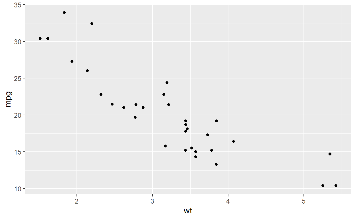
Three types of scatterplots representing different types of linear relationships:
- Strong Negative Linear Relationship:
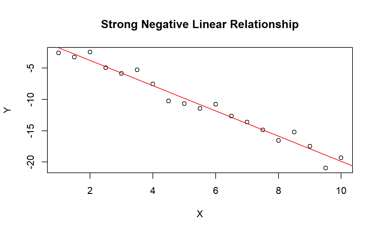
Figure 1: Strong Negative Linear Relationship
In this scatterplot, there is a strong negative linear relationship between the variables X and Y. As X increases, Y decreases in a linear fashion. The red line represents the linear regression line that best fits the data.
- No Linear Relationship:
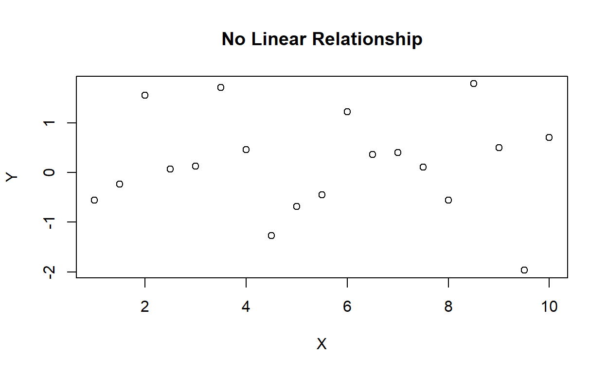
Figure 2: No Linear Relationship
In this scatterplot, there is no apparent linear relationship between the variables X and Y. The data points are scattered randomly with no clear pattern or trend.
- Strong Positive Linear Relationship:
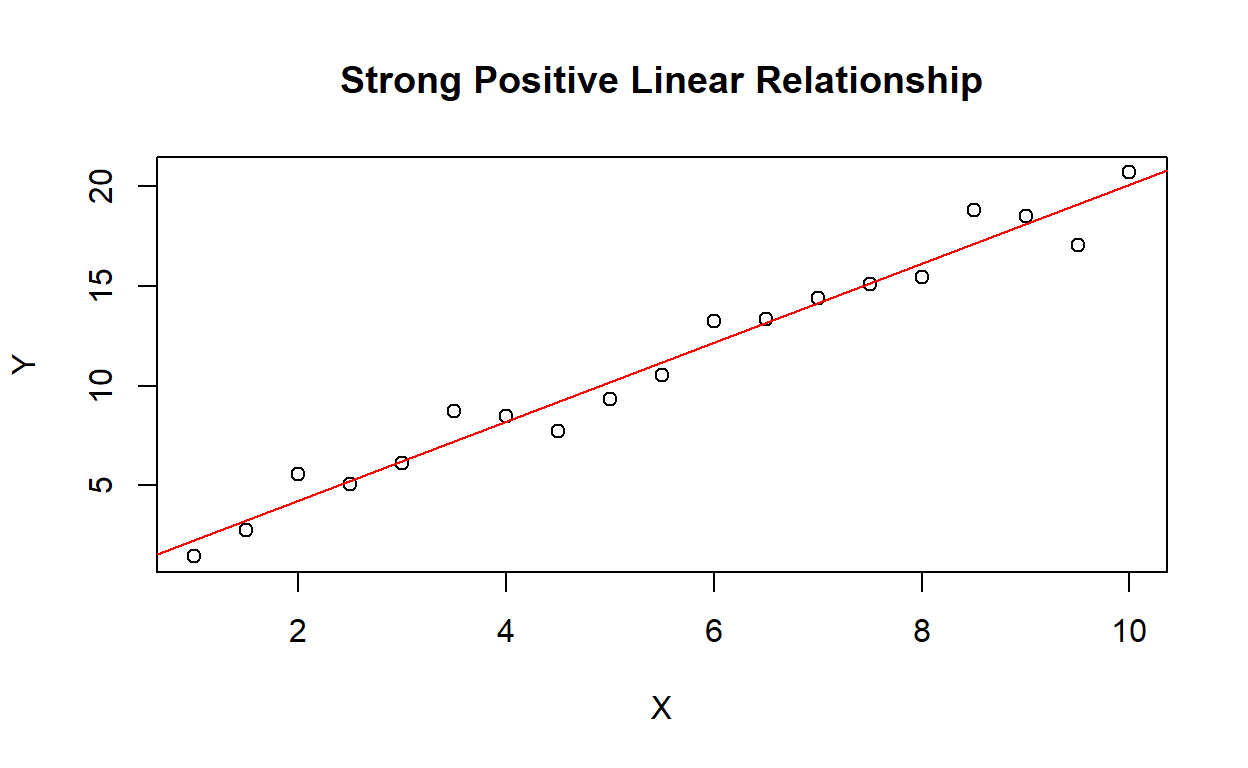
Figure 3: Strong Positive Linear Relationship
In this scatterplot, there is a strong positive linear relationship between the variables X and Y. As X increases, Y also increases in a linear fashion. The red line represents the linear regression line that best fits the data.
These scatterplots visually demonstrate different types of linear relationships: strong negative, no, and strong positive. They help us understand the direction and strength of the relationship between variables.
Correlation
Correlation is a measure of the strength and direction of the linear relationship between two variables. There are two ways to measure correlation: scatter diagram and linear correlation coefficient.
Linear Correlation Coefficient
The linear correlation coefficient (Pearson’s r) is a numerical measure of the strength and direction of the linear relationship between two variables. The value of r ranges from -1 to 1, where -1 indicates a strong negative correlation, 1 indicates a strong positive correlation, and 0 indicates no correlation.
The following formula can be used to calculate the correlation coefficient:
\[ r = \frac{\sum{(x_i - \bar{x})(y_i - \bar{y})}}{\sqrt{\sum{(x_i - \bar{x})^2}\sum{(y_i - \bar{y})^2}}}\ \ or\ r = \frac{S_{xy}}{\sqrt{S_{xx}\ \times\ S_{yy}}} \\ \\ \]
# Example correlation calculation
plot(mtcars$wt, mtcars$mpg, main = "Strong Negative Linear Relationship", xlab = "Weight", ylab = "MPG")
abline(lm(mtcars$mpg ~ mtcars$wt), col = "red")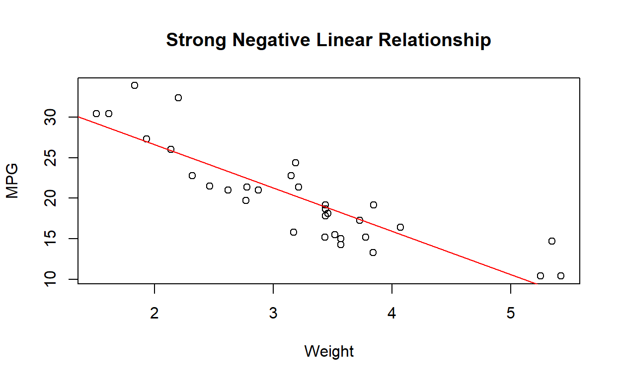
cor(mtcars$wt, mtcars$mpg)[1] -0.8676594The correlation coefficient (r) of -0.8676594 indicates a strong negative linear relationship between the variables being analyzed. This means that as one variable increases, the other variable tends to decrease.
Specifically, a correlation coefficient of -0.8676594 suggests that there is a strong inverse relationship between the variables, where higher values of one variable are associated with lower values of the other variable.
It is important to note that correlation does not imply causation, and further analysis is needed to determine the underlying factors driving this relationship.
Overall, the strong negative correlation coefficient indicates a robust and consistent pattern in the data, suggesting that changes in one variable are reliably associated with changes in the opposite direction in the other variable.
Positive, Negative, and No Correlation Examples
Positive Correlation
# Data
x <- c(2, 4, 6, 8, 10)
y <- c(3, 6, 9, 12, 15)

# Scatter plot
plot(x, y, main = "Positive Correlation", xlab = "X", ylab = "Y")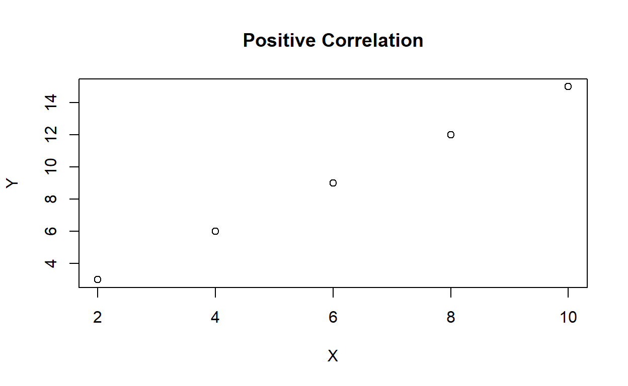
cor(x, y)[1] 1In this example, we have a positive correlation between the variables X and Y. As the value of X increases, the value of Y also increases. The scatter plot demonstrates a positive linear relationship between the variables.
Negative Correlation
# Data
x <- c(2, 4, 6, 8, 10)
y <- c(15, 12, 9, 6, 3)

# Scatter plot
plot(x, y, main = "Negative Correlation", xlab = "X", ylab = "Y")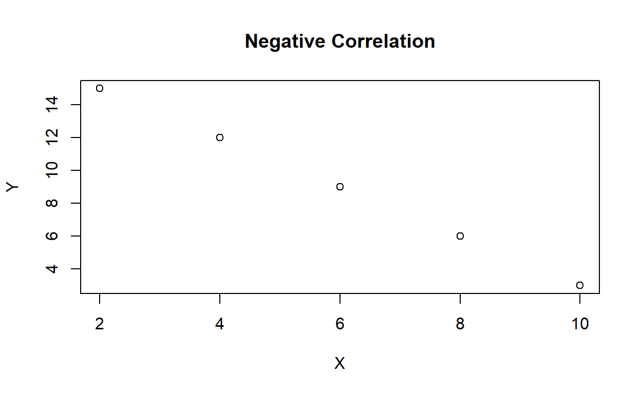
cor(x, y)[1] -1In this example, we have a negative correlation between the variables X and Y. As the value of X increases, the value of Y decreases. The scatter plot demonstrates a negative linear relationship between the variables.
No Correlation
# Data
x <- c(1, 2, 3, 4, 5)
y <- c(3, 1, 4, 2, 5)

# Scatter plot
plot(x2, y2, main = "No Correlation", xlab = "X", ylab = "Y")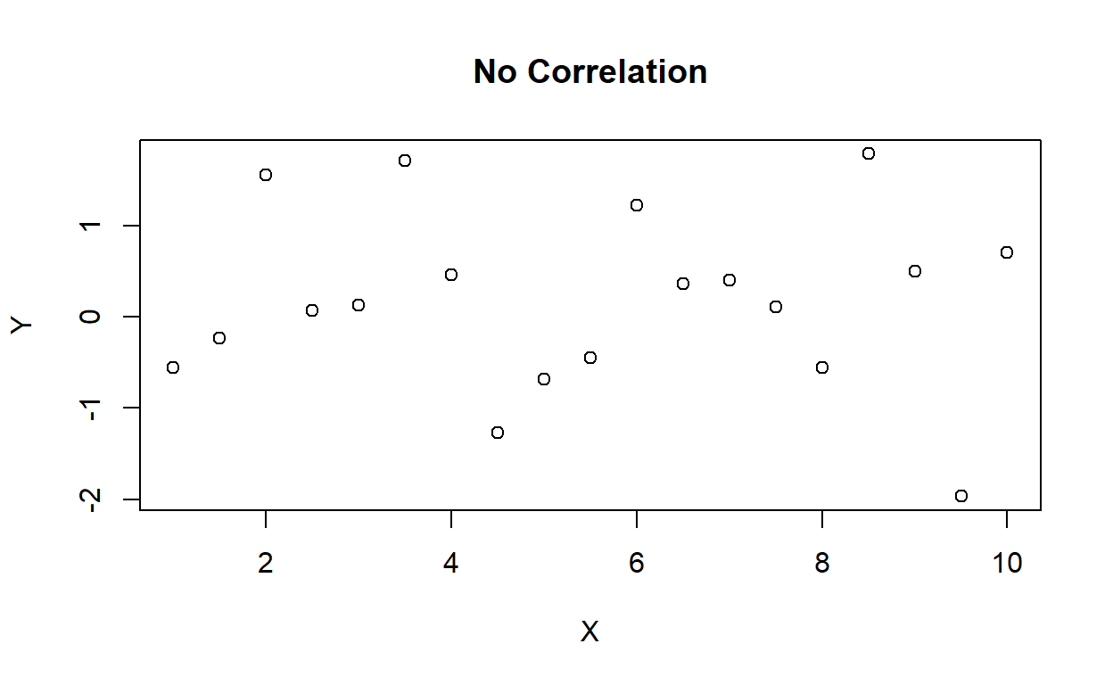
cor(x2, y2)[1] -0.04521122In this example, there is no discernible correlation between the variables X and Y. The scatter plot does not exhibit a clear pattern or trend, indicating no linear relationship between the variables.
In summary, correlation analysis helps us identify the strength and direction of relationships between variables. The examples provided demonstrate the concepts of positive, negative, and no correlation, as illustrated by the corresponding scatter diagrams.
To learn how to calculate the correlation coefficient using scietific calculator, you can watch the following videos in my YouTube Channel.
Simple Linear Regression
Simple linear regression is a statistical method used to model the relationship between a dependent variable (y) and an independent variable (x). The purpose of simple linear regression is to predict the value of the dependent variable based on the value of the independent variable.
Linear Regression Equation
The linear regression equation is \(y = \beta_0 + \beta_1x + \epsilon\), where \(\beta_0\) is the y-intercept, \(\beta_1\) is the slope, and \(\epsilon\) is the error term.
Call:
lm(formula = mpg ~ wt, data = mtcars)

Residuals:
    Min      1Q  Median      3Q     Max
-4.5432 -2.3647 -0.1252  1.4096  6.8727

Coefficients:
            Estimate Std. Error t value Pr(>|t|)
(Intercept)  37.2851     1.8776  19.858  < 2e-16 ***
wt           -5.3445     0.5591  -9.559 1.29e-10 ***
---
Signif. codes:  0 '***' 0.001 '**' 0.01 '*' 0.05 '.' 0.1 ' ' 1

Residual standard error: 3.046 on 30 degrees of freedom
Multiple R-squared:  0.7528,    Adjusted R-squared:  0.7446
F-statistic: 91.38 on 1 and 30 DF,  p-value: 1.294e-10
Estimating Linear Regression using Least Square Method
The least square method is a technique used to estimate the coefficients of the linear regression equation by minimizing the sum of the squared differences between the observed values and the predicted values.
Formulae
The formulae for estimating the slope and intercept of the linear regression equation using the least square method are:
# Example least square method
x <- mtcars$wt
y <- mtcars$mpg
x_bar <- mean(x)
y_bar <- mean(y)
beta1 <- sum((x - x_bar) * (y - y_bar)) / sum((x - x_bar)^2)
beta0 <- y_bar - beta1 * x_bar
cat("Slope (beta1):", beta1, "\n")
Slope (beta1): -5.344472 cat("Intercept (beta0):", beta0, "\n")Intercept (beta0): 37.28513 Coefficient of Determination
The coefficient of determination (R²) is a measure of the proportion of the variance in the dependent variable that is predictable from the independent variable. \(R^2\) ranges from 0 to 1, where 0 indicates that the independent variable does not explain any of the variance in the dependent variable, and 1 indicates that the independent variable explains all of the variance in the dependent variable.
# Example coefficient of determination
y_pred <- beta0 + beta1 * x
SSE <- sum((y - y_pred)^2)
SST <- sum((y - y_bar)^2)
R2 <- 1 - SSE / SST
cat("Coefficient of determination (R2):", R2, "\n")
Coefficient of determination (R2): 0.7528328 In conclusion, bivariate analysis is a crucial tool in understanding the relationship between two variables. By using correlation, simple linear regression, and the least square method, we can analyze the strength and direction of the relationship, as well as make predictions based on this relationship. The coefficient of determination helps us understand how well our model explains the variance in the dependent variable.
Assumptions of Simple Linear Regression
There are four assumptions of simple linear regression:
- Linearity: The relationship between the independent and dependent variables is linear.
- Independence: The observations are independent of each other.
- Homoscedasticity: The variance of the error term is constant across all levels of the independent variable.
- Normality: The error term is normally distributed.
Evaluating the Regression Model
There are several ways to evaluate the regression model:
Residual Analysis
Residuals are the differences between the observed values and the predicted values. Residual analysis is used to assess the validity of the regression model’s assumptions and identify potential outliers.
# Example residual plot
plot(model, which = 1)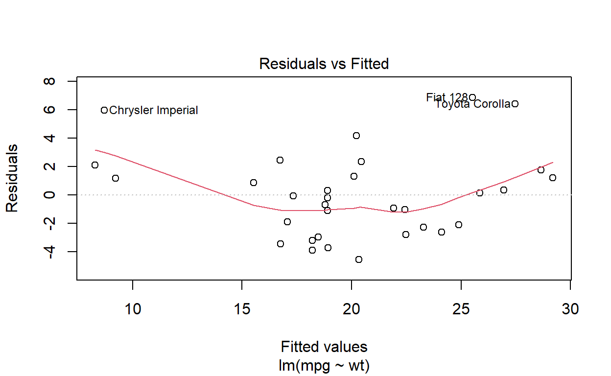
Hypothesis Testing for the Slope
Hypothesis testing is used to test the null hypothesis that there is no relationship between the independent and dependent variables. The test statistic is \(t = \frac{b_1 - 0}{SE(b_1)}\), where \(b_1\) is the estimated slope and \(SE(b_1)\) is the standard error of the slope.
Confidence Intervals for the Slope and Intercept
Confidence intervals are used to estimate the range of values for the population slope and intercept with a specified level of confidence (e.g., 95%).
# Example confidence intervals
confint(model)
2.5 % 97.5 %
(Intercept) 33.450500 41.119753
wt -6.486308 -4.202635Conclusion
In conclusion, bivariate analysis is a powerful tool for understanding the relationship between two variables and making predictions based on that relationship. By evaluating the regression model and its assumptions, we can ensure the validity of our findings and make data-driven decisions in various fields, such as marketing, finance, healthcare, and education. However, it is essential to be aware of the limitations of bivariate analysis and consider using multivariate analysis techniques when necessary to account for confounding variables and complex relationships.
Procedures in IBM Statistics SPSS
To run a correlation analysis in SPSS, follow these steps:
- Open SPSS and load your dataset.
- Click on “Analyze” in the top menu and select “Correlate” and then “Bivariate”.
- Select the variables you want to analyze by clicking on them in the left-hand column and then clicking the arrow button to move them to the right-hand column.
- Choose the correlation coefficient you want to use (e.g., Pearson, Spearman) and select any additional options you want to include (e.g., significance levels).
- Click “OK” to run the analysis.
To run a simple linear regression analysis in SPSS, follow these steps:
- Open SPSS and load your dataset.
- Click on “Analyze” in the top menu and select “Regression” and then “Linear”.
- Select the dependent variable you want to analyze by clicking on it in the left-hand column and then clicking the arrow button to move it to the “Dependent” box.
- Select the independent variable(s) you want to include by clicking on them in the left-hand column and then clicking the arrow button to move them to the “Independent(s)” box.
- Choose any additional options you want to include (e.g., confidence intervals, standardized coefficients).
- Click “OK” to run the analysis.
I hope this helps! Let me know if you have any other questions.
Examples
Correlation Analysis
Here’s an example of correlation analysis using SPSS output:
Correlations
             Height   Weight   Age
Height       1.000    0.780    0.432
Weight       0.780    1.000    0.658
Age          0.432    0.658    1.000

N = 100
In this example, the correlation matrix shows the correlations between three variables: Height, Weight, and Age. The correlation coefficient ranges from -1 to 1, where a value of 1 indicates a perfect positive correlation, 0 indicates no correlation, and -1 indicates a perfect negative correlation.
Based on the SPSS output, we can observe the following correlations:
- Height and Weight have a strong positive correlation of 0.780.
- Height and Age have a moderate positive correlation of 0.432.
- Weight and Age have a moderate positive correlation of 0.658.
The sample size (N) for this analysis is 100.
This SPSS output provides valuable information about the relationships between variables and helps in understanding the strength and direction of the correlations.
Simple Linear Regression Analysis
Here’s an example of simple linear regression analysis using SPSS output:
Model Summary
Model   R     R Square   Adjusted R Square   Std. Error of the Estimate
1       0.783 0.613      0.603               3.521

ANOVA
                Sum of Squares   df   Mean Square   F       Sig.
Regression      840.596          1    840.596       60.109  <0.001
Residual        531.404          28   18.979
Total           1372.000         29

Coefficients
                    Unstandardized Coefficients   Standardized Coefficients
Model               B          Std. Error         Beta          t       Sig.
(Constant)          6.210      3.054                            2.033   0.052
Height              0.780      0.100              0.783         7.755   <0.001
In this example, the simple linear regression analysis is performed to examine the relationship between two variables: Height and Weight.
The Model Summary section provides information about the overall fit of the regression model. The R value represents the correlation between the predicted and observed values, indicating the strength of the relationship. The R Square value (0.613) indicates that 61.3% of the variance in the dependent variable (Weight) is explained by the independent variable (Height). The Adjusted R Square value (0.603) takes into account the degrees of freedom and adjusts the R Square value accordingly. The Std. Error of the Estimate (3.521) represents the average error or residual between the predicted and observed values.
The ANOVA table shows the results of the analysis of variance. The Regression row provides information about the regression model’s overall performance. The Sum of Squares (840.596) represents the explained variance, while the Residual row represents the unexplained variance. The F value (60.109) indicates the significance of the regression model, and the Sig. value (<0.001) indicates that the regression model is statistically significant.
The Coefficients table provides information about the regression coefficients. The Unstandardized Coefficients represent the intercept (Constant) and the slope (Height). The Standardized Coefficients (Beta) show the standardized effect of the independent variable (Height) on the dependent variable (Weight). The t value and Sig. value indicate the significance of each coefficient.
This SPSS output provides important information about the regression model’s fit, significance, and the relationship between the independent and dependent variables.
More learning videos on this topic is available here: